This blog aims to implement some important Machine Learning, Deep Learning, Natural Language Processing, Large Language Models related algorithms from scratch, which can help people get deeper understanding about how these algorithms work in real code.
- Classic Machine Learning algorithms
- Deep Learning algorithms
- CV algorithms
- NLP algorithms
- LLM algorithms
- Mathematics
- References
Classic Machine Learning algorithms
K-means
Steps:
- Clusters the data into k groups where k is predefined.
- Select k points at random as cluster centers.
- Assign objects to their closest cluster center according to the Euclidean distance function.
- Calculate the centroid or mean of all objects in each cluster.
- Repeat steps 2, 3 and 4 until the same points are assigned to each cluster in consecutive rounds.
Implementation:
1
2
3
4
5
6
7
8
9
10
11
12
13
14
15
16
17
18
19
20
21
22
23
24
25
26
27
28
29
30
31
32
33
34
35
36
37
38
39
40
41
42
43
44
45
46
import numpy as np
def cal_dist(vector1, vector2):
# euclidian distance
eucl_dist = np.sqrt(np.sum((vector1 - vector2)**2))
return eucl_dist
def k_means(data, k):
n_samples, n_shape = data.shape
# random initialize centroids
centroid_index = np.random.choice(range(n_samples), k)
centroid_coords = data[centroid_index]
# label of each data point
labels = [-1] * n_samples
# iterate until centroid no longer change
while True:
for i in range(n_samples):
min_dist = float("inf")
min_cluster_idx = -1
for j in range(k):
dist = cal_dist(data[i], centroid_coords[j])
if dist < min_dist:
min_dist = dist
min_cluster_idx = k
# update cluster index for each point
label[i] = min_cluster_idx
# flag indicate if the centroid change of not: stop condition for while loop
centroid_update = False
# recalculate the centroids
for i, centroid in enumerate(centroid_coords):
# gather all data points for each cluster
cluster_points = []
for k in range(n_samples):
if label[k] == i:
cluster_points.append(data[k])
cluster_points = np.concatenate([cluster_points], axis=1)
# calculate new centroid
new_centroid_coord = np.mean(cluster_points, axis=0)
# see if the centroid change for each cluster
if cal_dist(centroid, new_centroid_coord) > 1e-5:
centroid_coords[i] = new_centroid_coord
centroid_update = True
if not centroid_update:
break
return labels
KNN implementation
1 | class kNN(): |
Logistic regression
NumPy implementation:
1 | # https://blog.51cto.com/u_15661962/5531479 |
Linear Regression
NumPy implementation for multiple linear regression (two or more features for each data point), simple linear regression (only one feature for each data point)
reference:
1 | import numpy as np |
Activation Functions
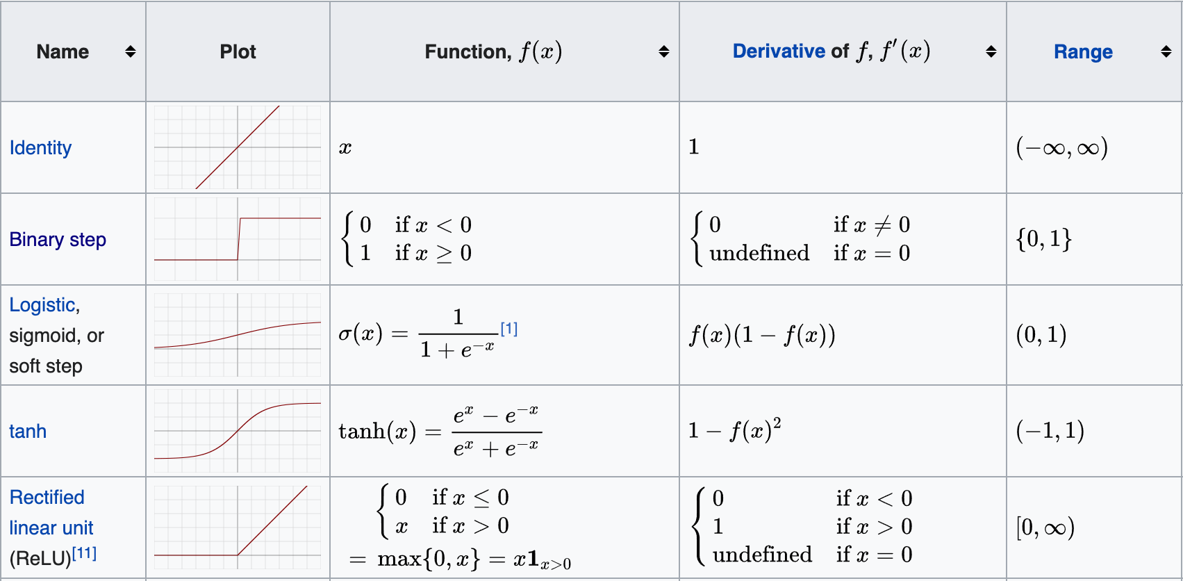
sigmoid (value from 0 to 1)
1
2
3import numpy as np
def sigmoid(x):
return 1 / (1 + np.exp(-x))ReLU (from 0 to infinity)
1
2
3
4
5def relu(x):
if x < 0:
return 0
else:
return xLeaky ReLU
1
2
3def leaky_relu(x, alpha=0.01):
"""Compute the Leaky ReLU activation."""
return max(alpha * x, x)tanh (from -1 to 1)
1
2
3import numpy as np
def tahn(x):
return (np.exp(x)-np.exp(-x)) / (np.exp(x) + np.exp(-x))Softmax (from 0 to 1)
1
2
3
4
5import numpy as np
def softmax(x):
# assumes x is a vector
x = x - np.max(x) # to avoid overflow
return np.exp(x) / np.sum(np.exp(x))GLU (Gated Linear Units) activation function

1
2
3
4
5
6
7
8
9import torch.nn as nn
class GLU(nn.Module):
def __init__(self, in_size):
super().__init__()
self.linear1 = nn.Linear(in_size, in_size)
self.linear2 = nn.Linear(in_size, in_size)
def forward(self, x):
return self.linear1(x) * self.linear2(x).sigmoid()Sigmoid Linear Unit (SiLU/swish) activation function

1 | import numpy as np |
Loss Functions
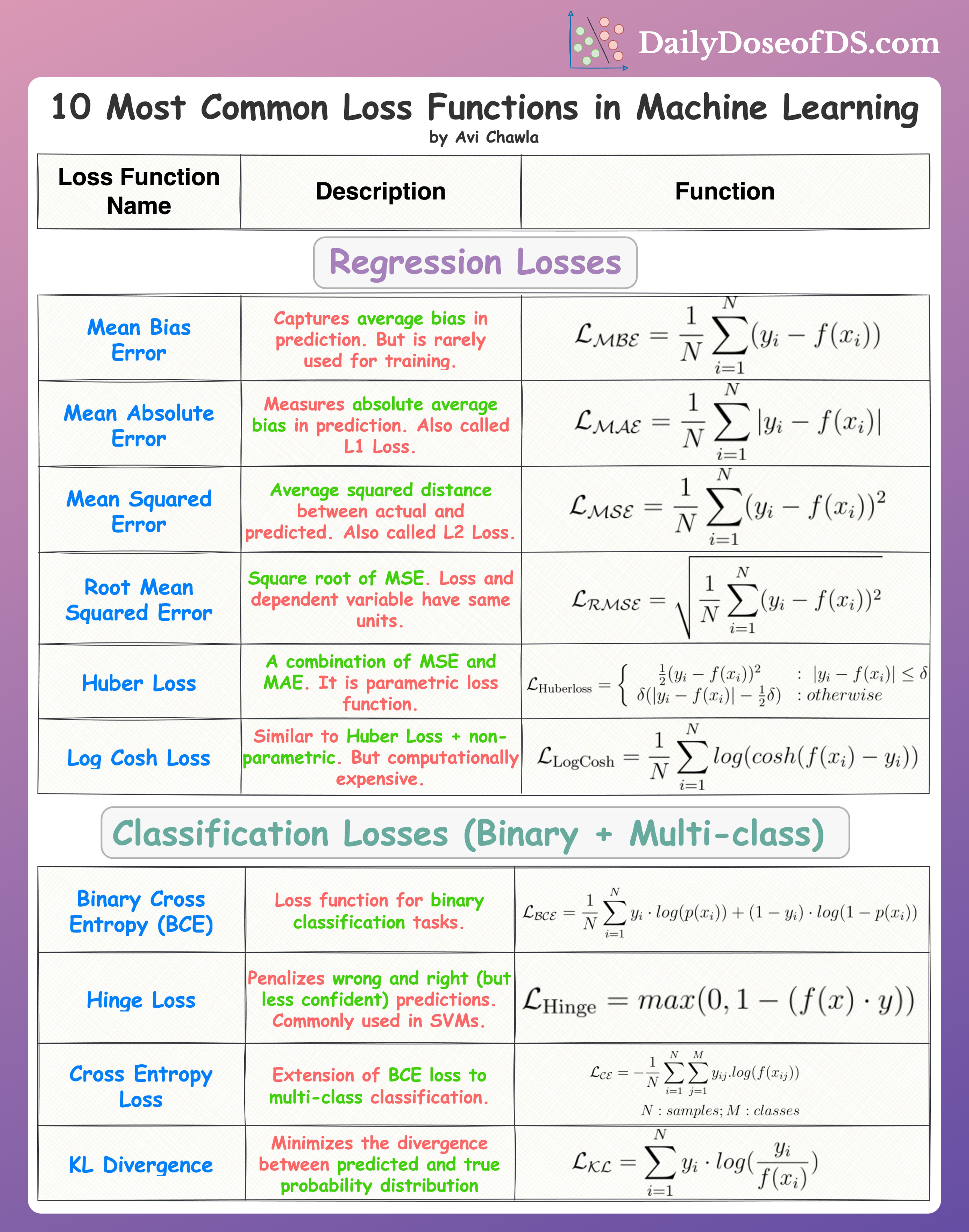
Binary Cross Entropy Loss
1 | import numpy as np |
Categorical Cross Entropy Loss
1 | import numpy as np |
KL divergence
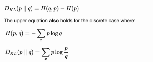
1 | import numpy as np |
Evaluation metrics
Recall, Precision, F1, accuracy

1 | ground_truth = [0, 0, 0, 0, 1, 0, 1, 0, 0, 1, 0, 1, 0, 0, 1, 0, 1] |
Marco & Micro average recall/precision
A macro-average will compute the metric independently for each class and then take the average (hence treating all classes equally), whereas a micro-average will aggregate the contributions of all classes to compute the average metric. In macro averaging, we compute the performance for each class, and then average over classes. In micro averaging, we collect the decisions for all classes into a single confusion matrix, and then compute precision and recall from that table.
In a multi-class classification setup, micro-average is preferable if you suspect there might be class imbalance (i.e you may have many more examples of one class than of other classes).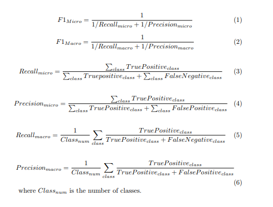
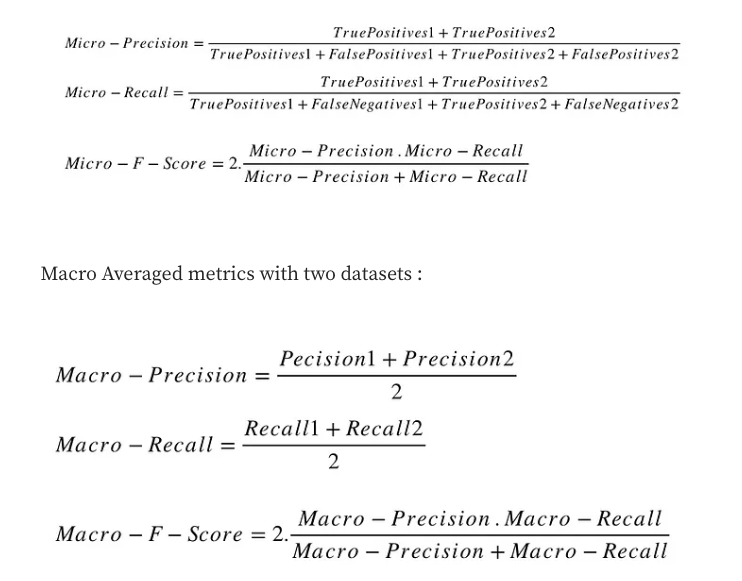
Macro-averaged metrics are used when we want to evaluate systems performance across on different datasets.
Micro-averaged metrics should be used when the size of datasets are variable.
ROC and AUC
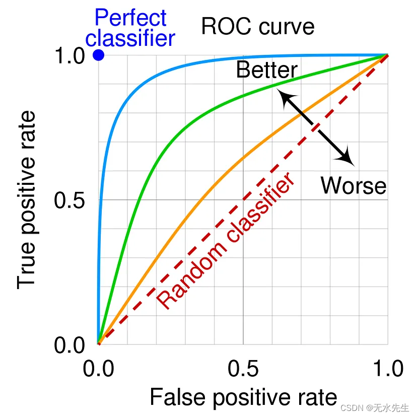
A receiver operating characteristic curve, or ROC curve, is a graphical plot that illustrates the performance of a binary classifier model (can be used for multi class classification as well) at varying threshold values. The ROC curve is the plot of the true positive rate (TPR) against the false positive rate (FPR) at each threshold setting.

AUC stands for “Area under the ROC Curve.” That is, AUC measures the entire two-dimensional area underneath the entire ROC curve (think integral calculus) from (0,0) to (1,1). AUC ranges in value from 0 to 1. A model whose predictions are 100% wrong has an AUC of 0.0; one whose predictions are 100% correct has an AUC of 1.0.
BLEU score
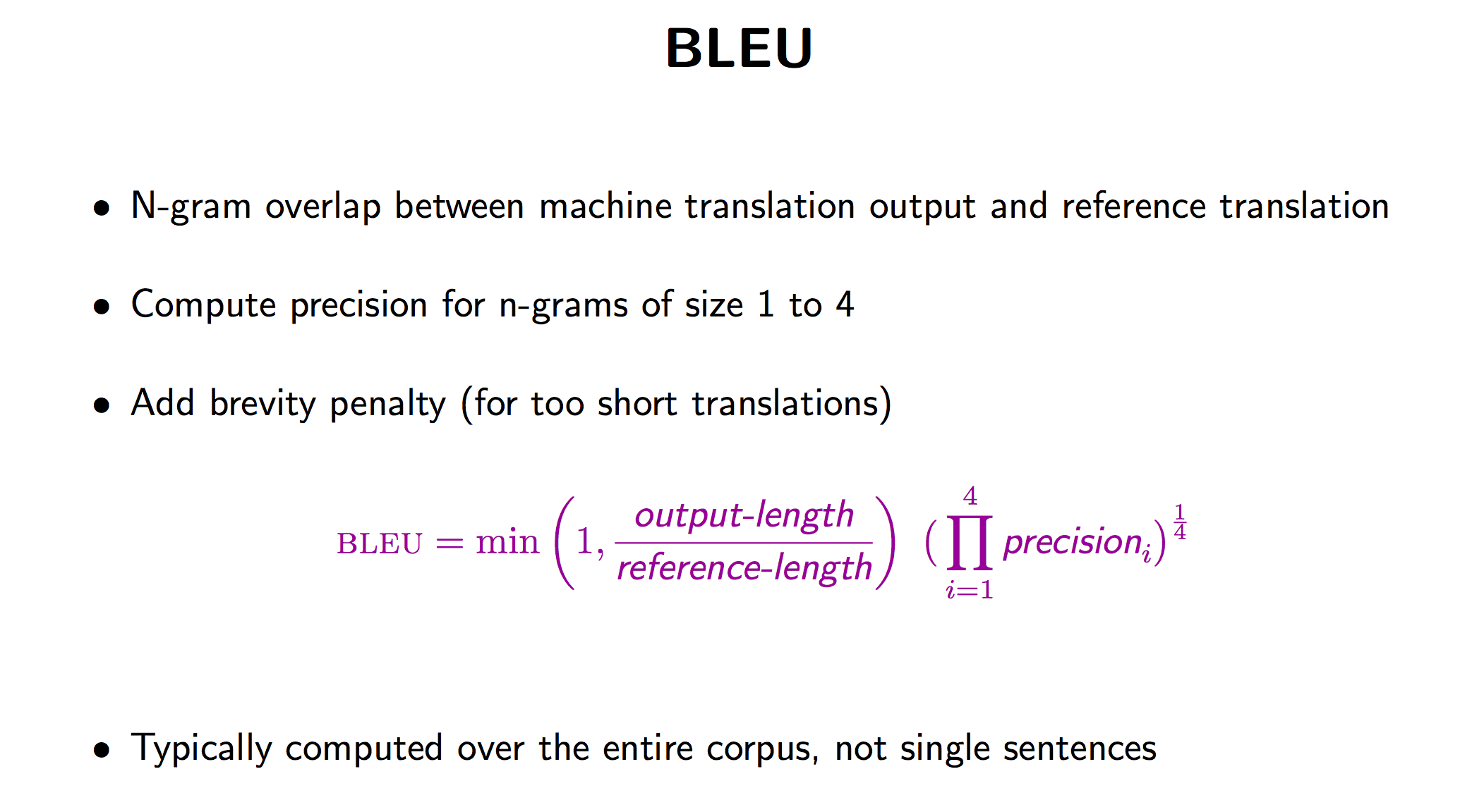
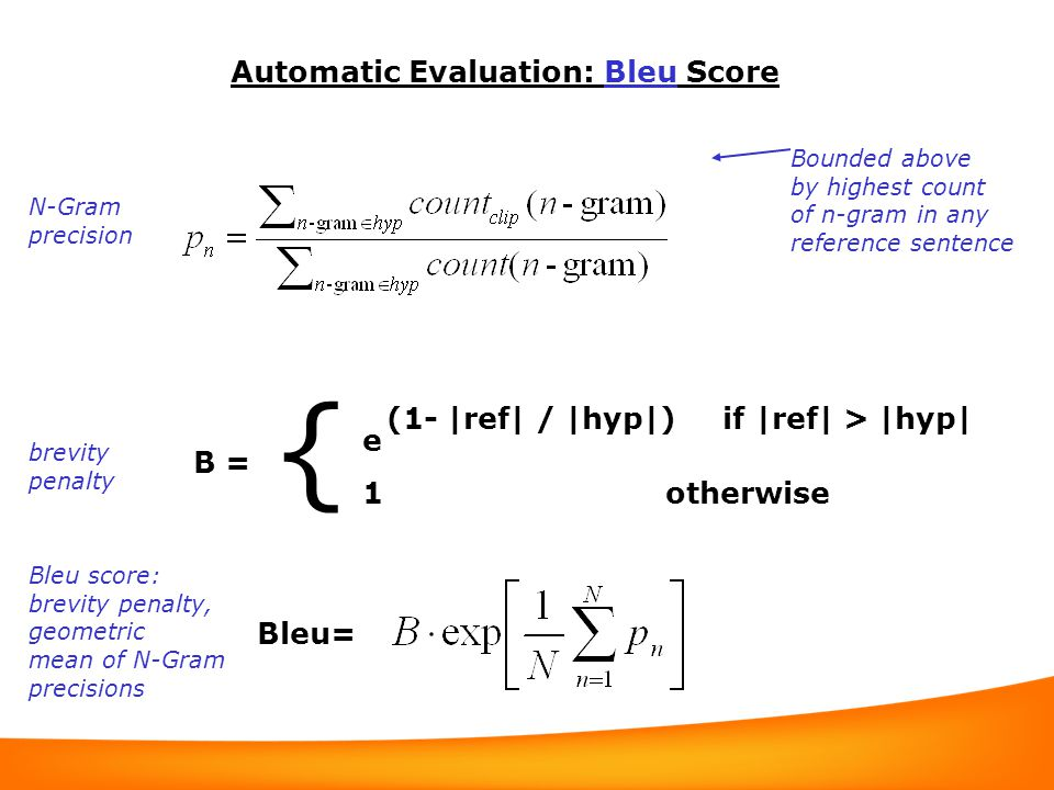
BLEU (bilingual evaluation understudy) is an algorithm for evaluating the quality of text which has been machine-translated from one natural language to another. BLEU’s output is always a number between 0 and 1. This value indicates how similar the candidate text is to the reference texts, with values closer to 1 representing more similar texts.
Rouge score
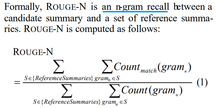
ROUGE, or Recall-Oriented Understudy for Gisting Evaluation, is a set of metrics and a software package used for evaluating automatic summarization and machine translation software in natural language processing. The metrics compare an automatically produced summary or translation against a reference or a set of references (human-produced) summary or translation. ROUGE metrics range between 0 and 1, with higher scores indicating higher similarity between the automatically produced summary and the reference.
- ROUGE-N: Overlap of n-grams between the system and reference summaries.
- ROUGE-L: Longest Common Subsequence (LCS) based statistics. Longest common subsequence problem takes into account sentence-level structure similarity naturally and identifies longest co-occurring in sequence n-grams automatically.

Perplexity
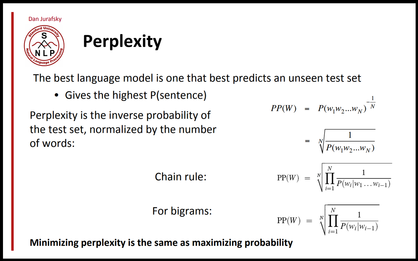
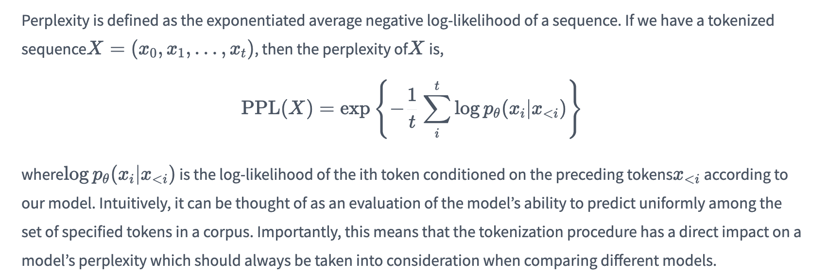
Perplexity (PPL) is one of the most common metrics for evaluating language models. Perplexity is defined as the exponentiated average negative log-likelihood of a sequence. Intuitively, it can be thought of as an evaluation of the model’s ability to predict uniformly among the set of specified tokens in a corpus. The lower perplexity means the model has better performance on the specific corpus.
1 | import torch |
MRR, MAP, NDCG
MRR
Mean Reciprocal Rank (MRR) is one of the metrics that help evaluate the quality of recommendation and information retrieval systems. Mean Reciprocal Rank (MRR) defines how good a retrieval system is to return a relevant result as the top result. To calculate the MRR, multiple queries are invoked. If all of these queries return a relevant document at the top, the score will be 1.0.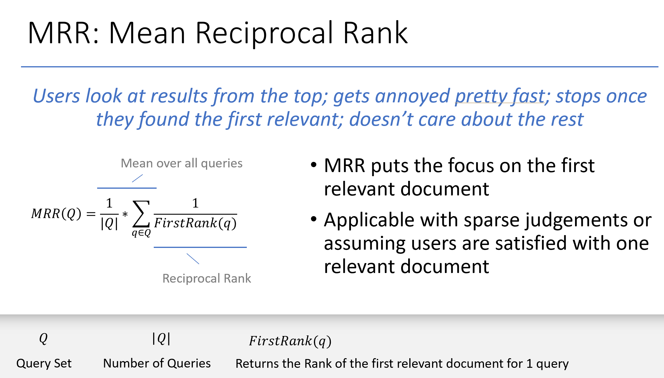
MAP
The disadvantage of MRR is that only the top document is considered. Other use cases like comparative questions in Question Answering scenarios require multiple relevant documents. Mean Average Precision (MAP) addresses this shortcoming by considering the order of the returned items. To calculate this score, three steps are taken:- Calculate precision
- Calculate average precision for K
- Calculate mean average precision for sample of queries
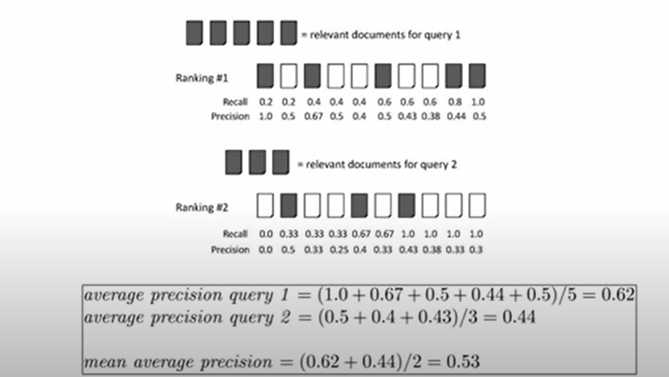
As for MRR, multiple queries are run. Instead of calculating the Recall, Precision is computed by using relevant and non-relevant documents from the returned lists (not the complete dataset).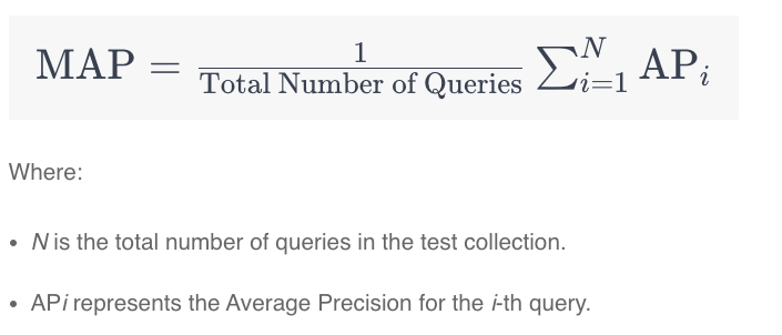
Average Precision (AP) is a widely used metric in information retrieval that quantifies the quality of a retrieval system’s ranked results for a single query. Unlike precision, which considers the entire ranked list of retrieved items, AP focuses on how well relevant items are ranked within that list. It measures the area under the precision-recall curve for a single query.
AP is calculated as follows:
- First, consider a query that retrieves a set of items.
- Compute the precision for each position where a relevant item is retrieved in the ranked results list.
- Average these precision values, but only for the positions where relevant items were retrieved.
- CG, DCG, NDCG
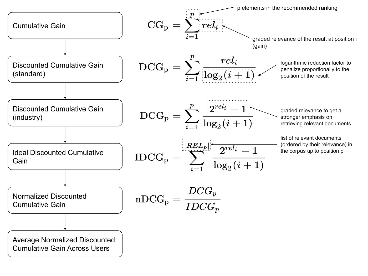
Discounted cumulative gain (DCG) is a measure of ranking quality which is often presented in its normalized and more easily interpretable form, known as Normalized DCG (nDCG or NDCG). In information retrieval, NDCG is often used to measure effectiveness of search engine algorithms and related applications.
nDCG implementation:
1 | import numpy as np |
Cross Validation
K-fold cross validation is a resampling technique used to evaluate the performance of machine learning models. It works by splitting the dataset into k folds, and then training the model on k-1 folds and testing it on the remaining fold. This process is repeated k times, with each fold being used as the test set once. The results are typically averaged to obtain a more robust estimate of your model’s performance.
1 | # k-fold cross validation implementation |
Deep Learning algorithms
Batch Normalization
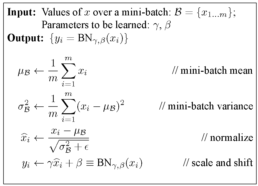
Why normalization?
The phenomenon by which the distributions of internal nodes (neurons) of a neural network change is referred to as Internal Covariate Shift. And we want to avoid it because it makes training the network slower, as the neurons are forced to re-adjust drastically their weights in one direction or another because of drastic changes in the outputs of the previous layers.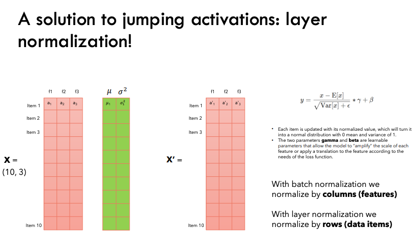
PyTorch implementation
1
2
3
4
5
6
7
8
9
10
11
12
13
14
15
16
17
18
19
20
21
22
23
24
25
26
27
28
29
30
31
32
33
34
35
36
37
38import torch
import numpy as np
def batchnorm_forward(x, gamma, beta, eps=1e-5):
N, D = x.shape # N is the batch size, D is the hidden size of each sample in batch
sample_mean = x.mean(axis=0) # shape [1, D]
sample_var = x.var(axis=0) # shape [1, D]
std = np.sqrt(sample_var + eps)
x_centered = x - sample_mean
x_norm = x_centered / std
out = gamma * x_norm + beta
return out
# with moving_mean and moving_var for inference
def batch_norm(X, gamma, beta, moving_mean, moving_var, eps, momentum):
'''
# X: (N, D) N is the batch size, D is the hidden size of each sample in batch
# The scale parameter and the shift parameter (model parameters) are
# initialized to 1 and 0, respectively
gamma = nn.Parameter(torch.ones(D,))
beta = nn.Parameter(torch.zeros(D,))
# The variables that are not model parameters are initialized to 0 and
# 1
moving_mean = torch.zeros(shape)
moving_var = torch.ones(shape)
'''
# test stage
if not torch.is_grad_enabled():
X_hat = (X - moving_mean) / torch.sqrt(moving_var + eps)
else: # training
mean = X.mean(dim=0)
var = ((X-mean)**2).mean(dim=0) # var = X.var(dim=0)
X_hat = (X - mean) / torch.sqrt(var + eps)
## update the mean and variance using moving average
moving_mean = (1.0 - momentum) * moving_mean + momentum * mean
moving_var = (1.0 - momentum) * moving-var + momentum * var
Y = gamma * X_hat + beta # scale and shift
return Y, moving_mean.data, moving_var.dataNumPy implementation
1
2
3
4
5
6
7
8
9
10
11
12
13
14import numpy as np
def batchnorm_forward(x, scales,, bias, eps=1e-5):
mean = x.mean(axis=0) # Shape = (w, h, c)
var = x.var(axis=0)
std = np.sqrt(var+ eps) # shape = (w, h, c)
# eps is used to avoid divisions by zero
# Compute the normalized input
x_norm = (x - mean) / std # shape (batch, w, h, c)
# Output = scale * x_norm + bias
if scales is not None:
x_norm *= scales # Multiplication for scales
if bias is not None:
x_norm += bias # Add bias
return x_norm
Layer Normalization

Explanation:
A well-known explanation of the success of LayerNorm is its re-centering and re-scaling invariance property. The former enables the model to be insensitive to shift noises on both inputs and weights, and the latter keeps the output representations intact when both inputs and weights are randomly scaled.
Numpy implementation
1
2
3
4
5
6import numpy as np
def layer_norm(x, g, b, eps: float = 1e-5):
mean = np.mean(x, axis=-1, keepdims=True)
variance = np.var(x, axis=-1, keepdims=True)
x = (x - mean) / np.sqrt(variance + eps) # normalize x to have mean=0 and var=1 over last axis
return g * x + b # scale and offset with gamma/beta paramsPytorch implementation
1
2
3
4
5
6
7
8
9
10
11
12
13import torch
import torch.nn as nn
# feature : (batch_size, seq_len, hidden_dim)
class LayerNorm(nn.Module):
def __init__(self, features, eps=1e-5):
super(LayerNorma, self).__init__()
self.a_2 = nn.Parameter(torch.ones(features))
self.b_2 = nn.Parameter(torch.zeros(features))
self.eps = eps
def farward(self, x):
mean = x.mean(-1, keepdim=True) # (batch_size, seq_len, 1)
std = x.std(-1, keepdim=True) # (batch_size, seq_len, 1)
return self.a_2 * (x-mean) / (std+self.eps) + self.b_2
Dropout
1 | class Dropout(): |
Optimizers
SGD (Stochastic Gradient Descent)
Advantages:
- Frequent updates of model parameters, converges in less time
- Requires less memory as no need to store values of loss functions
- May get new minima’s
Disadvantages: - High variance in model parameters
- May shoot even after achieving global minima
- To get the same convergence as gradient descent needs to slowly reduce the value of learning rate
Mini-Batch Gradient Descent (BGD)
Advantages:
- Frequently updates the model parameters and also has less variance
- Requires medium amount of memory
All types of Gradient Descent have some challenges: - May get trapped at local minima
- Choosing an optimum value of the learning rate. If the learning rate is too small than gradient descent may take ages to converge
- Have a constant learning rate for all the parameters. There may be some parameters which we may not want to change at the same rate
Momentum
Used in conjunction Stochastic Gradient Descent or Mini-Batch Gradient Descent, Momentum takes into account past gradients to smooth out the update.
This is seen in variable 𝑣, which is an exponentially weighted average of the gradient on previous steps. This results in minimizing oscillations and faster convergence.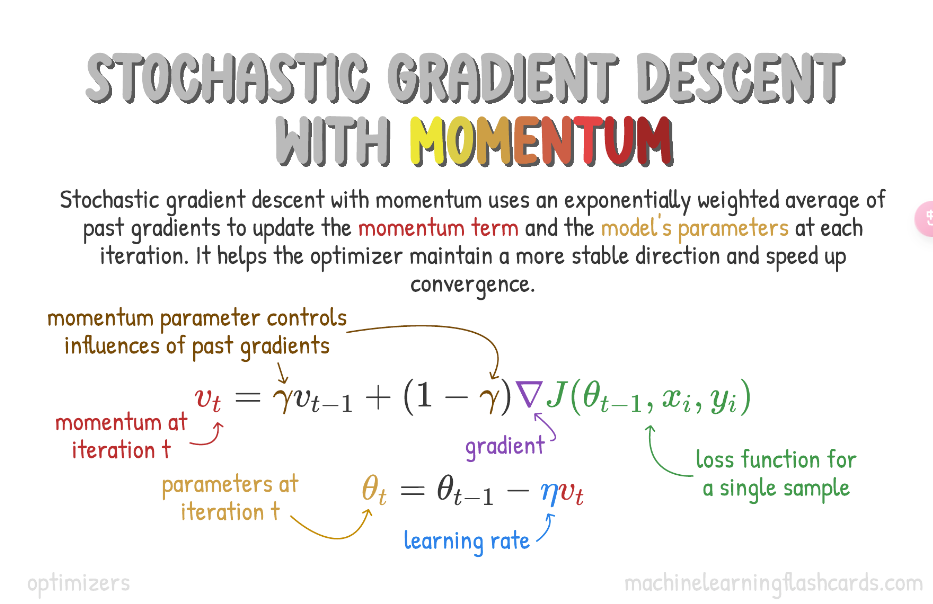
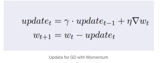
Compared with (minibatch) stochastic gradient descent the momentum method needs to maintain a set of auxiliary variables, i.e., velocity. It has the same shape as the gradients (and variables of the optimization problem). In the implementation below we call these variables states.
1 | def init_momentum_states(feature_dim): |
Adagrad (Adaptative Gradient)
Adagard optimizer changes the learning rate for each parameter at every time step. Particularly, it tends to assign higher learning rates to infrequent features, which ensures that the parameter updates rely less on frequency and more on relevance.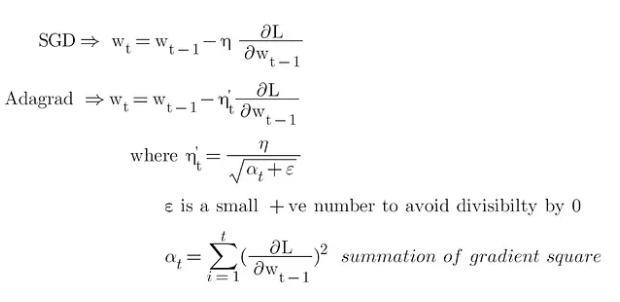
Advantages:
- Learning rate changes for each training parameters
- Don’t need to manually tune the learning rate
- Able to train on sparse data
Disadvantages: - Computationally expensive as a need to calculate the second order derivative
- The learning rate is always decreasing results in slow training
1 | def init_adagrad_states(feature_dim): |
Adadelta
Instead of accumulating all previously squared gradients, Adadelta limits the window of accumulated past gradients to some fixed size w.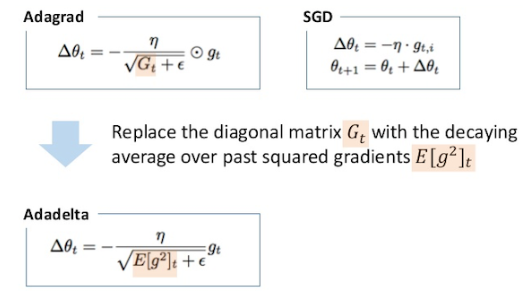
1 | def init_adadelta_states(feature_dim): |
RMSProp (Root Mean Square Propagation)
RMSProp is very similar to Adagrad insofar as both use the square of the gradient to scale coefficients. RMSProp shares with momentum the leaky averaging. However, RMSProp uses the technique to adjust the coefficient-wise preconditioner. The learning rate needs to be scheduled by the experimenter in practice.
1 | def init_rmsprop_states(feature_dim): |
Adam (Adaptive Moment Estimation)
Adam can be looked at as a combination of RMSprop and Stochastic Gradient Descent with momentum. Adam computes adaptive learning rates for each parameter. In addition to storing an exponentially decaying average of past squared gradients like Adadelta and RMSprop, Adam also keeps an exponentially decaying average of past gradients, similar to momentum.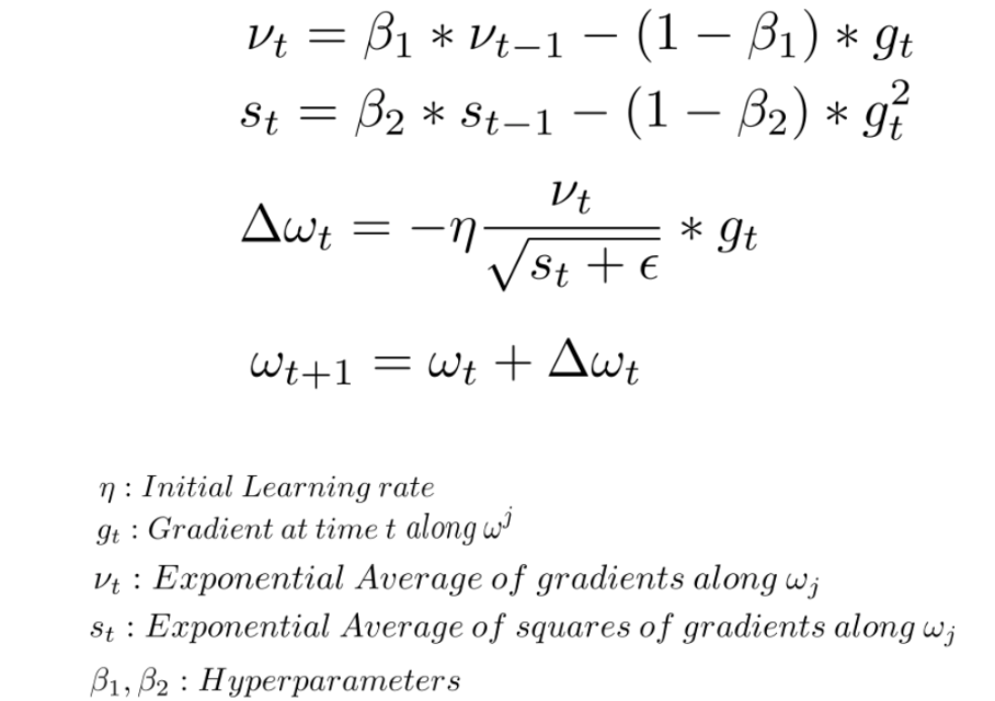
1 | def init_adam_states(feature_dim): |
Note: AdamW(Adam with decoupled weight decay)
CV algorithms
CNN
Components of CNN: Convolution, Pooling, Flatten, Fully connected layer
Basic PyTorch CNN implementation:
1 | class SimpleCNN(nn.Module): |
PyTorch implementation for Convolution and Pooling:
1 | def corr2d(image, kernel, padding_size, stride): #cross-correlation operation |
NumPy implementation of Convolution and Pooling
1 | def conv2d(image, num_filters, stride, kernel_size, padding=0): |
Patch Embedding
1 | # 2D image to patch embedding |
NLP algorithms
Basic Preprocessing
Here are the steps.
1 | # remove URLs |
Cosine similarity
NumPy Implementation
1 | import numpy as np |
python implementation
1 | def dot_product(A,B): |
TF-IDF
Terminology:
TF - Term Frequency, DF - Document Frequency, IDF - Inverse Document Frequency.
t — term (word), d — document (set of words), N — count of corpus, corpus — the total document set.
Formula:
TF(t,d) = count of t in d / number of words in d
DF(t) = the number of documents containing the term t
IDF(t) = N / DF(t)
To avoid IDF value explodes we take the log of IDF ==> IDF(t) = log( N / (DF(t) + 1) )
TD-IDF(t, d) = TF(t,d) * IDF(t)
1 | import numpy as np |
Sometimes we use TF-IDF for query-document retrieval task, in this case, we will calculate TF and IDF for each word in query according to different documents. Here is the example: blog
FastText
fastText is usually used to do classification tasks, it has two main improvements:
- used char-level n-gram as additional word embedding features
- used hierarchical softmax to reduce computation cost
1
2
3
4
5
6
7
8
9
10
11
12
13
14
15
16
17
18
19
20
21
22
23
24
25
26
27
28
29
30
31
32
33
34
35
36
37
38
39
40import torch
import torch.nn as nn
import torch.nn.functional as F
class FastText(nn.module):
def __init__(self, config):
super(FastText, self).__init__()
self.embedding_word = nn.Embedding(
config.vocab_size,
config.embed_size,
padding_idx = config.vocab_size-1
)
self.embedding_bigram = nn.Embedding(
config.ngram_vocab_size,
config.embed_size,
padding_idx = config.ngram_vocab_size-1
)
self.embedding_trigram = nn.Embedding(
config.ngram_vocab_size,
config.embed_size,
padding_idx = config.ngram_vocab_size-1
)
self.dropout = nn.Dropout(config.dropout_rate)
self.fc1 = nn.Linear(config.embed_size * 3, config.hidden_size)
self.fc2 = nn.Linear(config.hidden_size, config.num_classes)
def forward(self, x):
'''
:param x: x[0] (words), x[1] (bigram), x[2] (trigram): all have shape [batch_size, seq_length]
:return: [batch_size, num_classes] classification task
'''
embed_bow = self.embedding_word(x[0])
embed_bigram = self.embedding_bigram(x[1])
embed_trigram = self.embedding_trigram(x[2])
input = torch.cat((embed_bow, embed_bigram, embed_trigram), -1)
out = input.mean(dim=1)
out = self.dropout(out)
out = self.fc1(out)
out = F.relu(out)
out = self.fc2(out)
return out
RNN implementation
1 | class RNN(nn.Module): |
Absolute position embedding
1 | class PositionEncoding(nn.Module): |
Greedy search decoding
1 | # greedy decoder |
Beam search decoding
Beam Seach details: here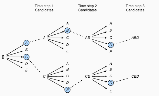
1 | import numpy as np |
LLM algorithms
LoRA (Low Rank Adaption) Implementation
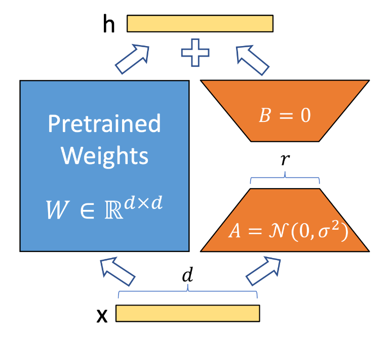
1 | import torch.nn as nn |
Autoregressive decoding
Decoder models generate tokens one by one during inference, e.g. GPT, Llama, BART, T5 etc. We can this autoregressive decoding and it is the main bottleneck of inference speed for decoder models.
Here is an sample implementation of this autoregressive decoding process:
1 |
|
Speculative Decoding
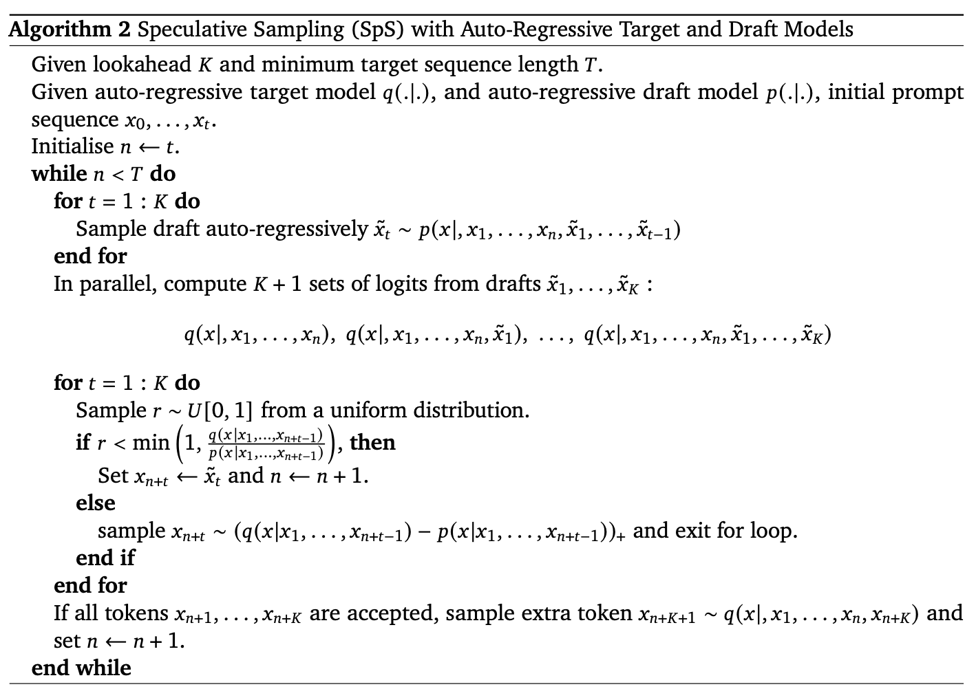
This technology is used in LLM inference stage to speed up Auto-regressive decoding steps.
Main idea: (source)
In speculative sampling, we have two models:
- A smaller, faster draft model
- A larger, slower target model
The idea is that the draft model speculates what the output is steps into the future, while the target model determines how many of those tokens we should accept.
The intuition behind speculative sampling is that certain strings of tokens (common phrases, pronouns, punctuation, etc …) are fairly easy to predict, so a smaller, less powerful, but faster draft model should be able to quickly predict these instead of having our slower target model doing all the work.
The algorithm is following:
- The draft model decodes K tokens in the regular autoregressive fashion.
- We get the probability outputs of the target and draft model on the new predicted sequence.
- We compare the target and draft model probabilities to determine how many of the K tokens we want to keep based on some rejection criteria. If a token is rejected, we resample it using a combination of the two distributions and don’t accept any more tokens.
- If all K tokens are accepted, we can sample an additional final token from the target model probability output.
As such, instead of decoding a single token at each iteration, speculative sampling decodes between 1 to K+1 tokens per iteration. If no tokens are accepted, we resample guaranteeing at least 1 token is decoded. If all K tokens are accepted, then we can also sample a final token from the target models probability distribution, giving us a total of K+1 tokens decoded.
Mathematics
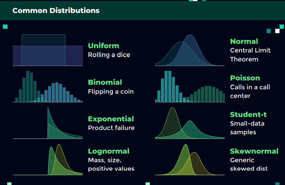
Different distributions
References
- https://www.cnblogs.com/wevolf/p/15195143.html
- https://lilianweng.github.io/posts/2021-05-31-contrastive/
- https://github.com/hkproj/pytorch-llama/tree/main
- https://arxiv.org/pdf/1910.07467.pdf
- https://towardsdatascience.com/optimizers-for-training-neural-network-59450d71caf6
- https://ml-cheatsheet.readthedocs.io/en/latest/optimizers.html#momentum
- https://arxiv.org/pdf/2211.15596.pdf
- https://spotintelligence.com/2023/09/14/mean-average-precision/
- https://www.kaggle.com/code/ajinkyaabhang/implementing-tpr-fpr-roc-auc-from-scratch
- https://ethen8181.github.io/machine-learning/model_selection/auc/auc.html
